Cheat sheet

Author @rihemebh Note that this cheat sheet is not completed yet please make your PR to contribute

Definitions

• Data Mining presents the discovery of knowledge (interesting information) from large amounts of data, by automatic methods

• Machine learning is a subfield of AI that focus on the study of algorithms built based on data in order to fuilfil a specific task. the algorithm performance could be improved with experience.

Example: hand writing recognition

• Task= recognition and classification of words written manually from images.
• Experience = a database of handwritten words with the appropriate classifications.
• Performance = The number of correctly classified words

ML VS DM

Data mining is designed to extract the rules from large quantities of data, while machine learning teaches a computer how to learn and comprehend the given parameters

Methodologies

KDD (by Ossama Fayyad - 1996)

KDD knowledge discovery process is iterative and interactive, comprises of nine steps :

1. Building up an understanding of the application domain
2. Choosing and creating a data set on which discovery will be performed
3. Preprocessing and cleansing
4. Data Transformation In this stage, the creation of appropriate data for Data Mining is prepared and developed. Techniques here incorporate dimension reduction( for example, feature selection and extraction and record sampling), also attribute transformation(for example, discretization of numerical attributes and functional transformation).
5. Prediction and description We are now prepared to decide on which kind of Data Mining to use, for example, classification, regression, clustering, etc.
6. choose the right Data Mining algo
7. Implement the algo
8. Evaluation
9. Using the discovered knowledge

SEMMA

1. Sample

   Extracts samples from a large data set, in numbers large enough to contain the important information, but small enough to be quickly manipulated.

2. Explore

   Exploring the data by looking for unforeseen anomalies in order to better understand the data.

3. Modify

   Modifies data by creating, selecting and transforming variables to focus on the model selection process.

4. Model

   Models the data by allowing the software to automatically search for a combination of data that reliably predicts the desired outcome

5. Assess Assesses the usefulness and reliability of the results of the Data Mining process and assesses how it will perform

CRISP-DM: CRoss-IndustryStandard Processfor Data Mining (By IBM)

1. Business Understanding

   Essential things to be determined in this phase:

   · Business Objectives

   · Data Mining Goals

   · Definition of project success criteria

2. Data Understanding

   Explore the data with the statistical method and data visualization.

3. Data hub building (Data Preparation)

   · Select Important Columns

   · Sampling Rows (Train Test Split, Cross-Validation)

   · Create or Derives new compound variables

   · Filter data (Filter Out Irrelevant data points)

   · Merging data sources (Data Aggregations)

   · Impute or Remove Missing value

   · Decide whether to remove or keep Outlier

4. Modelling

   Choose the right algorithm for modelling:

   Are you doing supervised learning or unsupervised learning?

   Which types are your problem? Regression? Classification?

   -> From there, you can determine your algorithm

5. Evaluation

6. Deployment

To know

	Meaning
Features	predictor variables
Class	Target variable
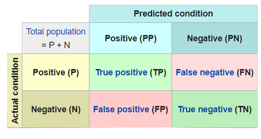
Overfitting	we talk about overfitting when a model has learned too much the particularities of each of the examples provided as an example. It then presents a very high success rate on the training data (which can reach up to 100%), but does not generalize well (less good performance on the test data).

Supervised Learning

Supervised learning is a type of machine learning that it is based on labeled or classified dataset to predict the label of new unkonw data.

How it works ?

Supervised learning uses a training set to teach models to yield the desired output. This training dataset includes inputs and correct outputs, which allow the model to learn over time. The algorithm measures its accuracy through the loss function, adjusting until the error has been sufficiently minimized. (IBM-2020)

When we need domain expert ?

We need an expert at the begining to put the correct labels on data.

Classification: When the data that we want to predict is discret (YES/NO , {1,2,3..} ..)

Regression: When the Data that we want to predict is continous (price, distance .. )

Libraries to use

• scikit-learn/sklearn
• keras

Decision Tree

// edit to add

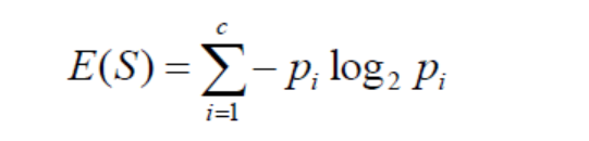
Entropy

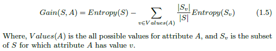
Information Gain

Bagging & Random Forest

// edit to add this part

K-NN

Predict the label of a data point by :

• Looking at the ‘k’ closest labeled data points
• Taking a majority vote

Choosing k

• Larger k= smoother decision boundary = less complex model
• Smaller k=more complex model=can lead to overfitting

Practice

Fit and predict

from sklearn.neighbors import KNeighbors

Classifierknn = KNeighborsClassifier(n_neighbors=6)
knn.fit(iris['data'], iris['target'])

X_new = np.array([[5.6, 2.8, 3.9, 1.1],       [5.7, 2.6, 3.8, 1.3],       [4.7, 3.2, 1.3, 0.2]])
prediction = knn.predict(X_new)

print('Prediction: {}’.format(prediction))
## output:
Prediction: [1 1 0]

Split and calculate performance with score()

from sklearn.model_selection import train_test_split
X_train, X_test, y_train, y_test =    train_test_split(X, y, test_size=0.3, random_state=21, stratify=y)
knn = KNeighborsClassifier(n_neighbors=8)
knn.fit(X_train, y_train)
y_pred = knn.predict(X_test)
print(\"Test set predictions:\\n {}\".format(y_pred))
# Output : Test set predictions: [2 1 2 2 1 0 1 0 0 1 0 2 0 2 2 0 0 0 1 0 2 2 2 0 1 1 1 0 0 1 2 2 0 0 2 2 1 1 2 1 1 0 2 1]

knn.score(X_test, y_test)

#Output: 0.9555555555555556

Naive bayes

Associate to each new instance the class that has the biggest probability. Naive Bayes classifier assumes that the features we use to predict the target are independent and do not affect each other. That’s why it is called naïve.

Bayes Formula: P(class| features) = P(Features|class) * P(class) / P(features)

• P(A|B) is the probability of hypothesis A given the data B. => posterior probability.

• P(B|A) is the probability of data B given that the hypothesis A was true. => Likelihood probability

• P(A) is the probability of hypothesis A being true (regardless of the data). This is called the prior probability of A.

• P(B) is the probability of the data (regardless of the hypothesis).

How it works?

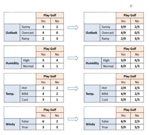
We will take the example of the famous weather dataset

• Create a frequency and likelihood table for Every features against all classes

We have 3 rules for the classification

• Majority rule

=> We choose the class that has the maximum P(class)

• Maximum rule

=> We choose the class that has the maximum P(class|feature)

• Bayes rule

=> We choose the class that has the maximum P(class|feature)* P(class)

Practice with scikit-learn

from sklearn import naive_bayes

nb = naive_bayes.MultinomialNB(fit_prior=True)
# Training
nb.fit(irisData.data[:], irisData.target[:])
# Prediction
p31 = nb.predict([irisData.data[31]])

plast = nb.predict([irisData.data[-1]])

predicted_results = nb.predict(irisData.data[:])
print("Prediction results", predicted_results)
print("Actual results", irisData.target)

Calculate performance

import numpy as np
# Training
nb.fit(irisData.data[:], irisData.target[:])
# Predict
P = nb.predict(irisData.data[:])

Y = irisData.target

#Calculate score
#Method 1
ea = 0
for i in range(len(irisData.data)):
  if (P[i] != Y[i]):
    ea = ea+1
print("Error using sum function :",ea/len(irisData.data))

# Method 2

#Non-zero values represent errors made by the model. So we can use the count_nonzero() function from the numpy package.
print("Error using numpy :",np.count_nonzero(P-Y)/len(irisData.data))

# Method 3

print("Accuracy : ",nb.score(irisData.data,Y))

Test

Cross Validation

The original sample is divided into k samples, then one of the k samples is selected as the validation set while the k-1 other samples constitute the training set. After learning, a validation performance can be calculated. Then the operation is repeated by selecting another validation sample from among the predefined blocks. At the end of the procedure we thus obtain performance scores, one per block.

The mean and standard deviation of performance scores can be calculated to estimate bias and variance in validation performance.

Cross Validation Practice

from sklearn.model_selection import cross_val_score
from sklearn.linear_model import LinearRegression
reg = LinearRegression()
cv_results = cross_val_score(reg, X, y, cv=5)
print(cv_results)

# different performance scores : [ 0.63919994  0.71386698  0.58702344  0.07923081 -0.25294154]
np.mean(cv_results)
# the mean result : 0.35327592439587058

Train Test Split

We split our dataset to 2/3 for training and 1/3 for test

=> Calculate performance on a new data

Why we use it?

• When the dataset is large it is very expensive to use other test methods like cross validation also we have enough data for our model to learn from and test with new data will be more efficient and very close to the real-life performance

Measuring model performance

Gerenally our metric is " Accuracy " : The more it is higher the more we have better performance. But this isn't the case when we are working with unbalanced datasets when there is significant disparity between the number of positive and negative labels which is the most common case in the real life problems that's why we need to have other metrics

Confusion matrix

• It is generally used with binary classification: (True/Flase , Spam/NotSpam .. )

Metric	Meaning
Accuracy	General metric : Fraction of correct predictions: number of correctly classified instances / total number of instances
Precision	When the cost of false positive is high : TP/ TP + FP
Recall	When the cost of false negative is high : TP/ TP + FN
F-Score	A measure that combines precision and recall is their harmonic mean : 𝐹=2∗𝑃𝑟e𝑐𝑖𝑠𝑖𝑜𝑛∗𝑅ecall / Precision+𝑅ecall

We should note that it works well with non binary classification: See this article for more details

Unsupervised learning

Unsupervised learning is based on unlabled data, it uses machine learning algorithms to analyse and cluster those data without human intervention

When we need domain expert ?

Since we are dealing with unlabeled data so the most critical part that need domain expert is the validation of the clusturing

Clusturing : Clustering is a data mining technique which groups unlabeled data based on their similarities or differences.

We optimize the clusturing by calculating the intercluster (between 2 clusters) + intracluster (within a cluster) distances Similarity: Similarity is the fact that 2 instances are similar depending on the metric we use. The larger the measure, the more similar the points. the metric used to calculate similarity is the distance The calculation of the distance depends on the data type:

<-- edit to complete this part -->

Types	Distance
continous	1. Normalisation : transform data into values between [0..1]

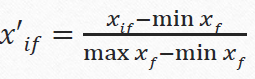
-- Xif is the value of the feature "f" in the line "i"

1. Standarisation

Z-score=

where Sf, mf =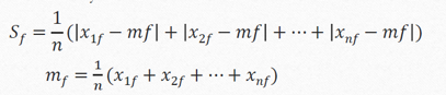

1. Distance :

• Minkow

• Menhaten

• Euclidien | | Binary | | | Nominal | | | Ordinal | | | Mixed | |

Clusturing Algorithms

K-means

K-Medoides

Hierarchical Algorithms

AGNES

DIANA

Implementation : https://github.com/rihemebh/ML-Labs/blob/main/unspervised_learning/diana.py

Performance